Diffusion 2D Unconditional Example

This notebook demonstrates how to train and sample from a diffusion model on a 2D toy dataset using JAX and Flax. We will cover data generation, model definition, training, sampling, and visualization.

1. Environment Setup

In this section, we set up the notebook environment, import required libraries, and configure JAX for CPU or GPU usage.

# Load autoreload extension for development convenience
%load_ext autoreload
%autoreload 2

The autoreload extension is already loaded. To reload it, use:
  %reload_ext autoreload

try: #check if we are using colab, if so install all the required software
    import google.colab
    colab=True
except:
    colab=False

if colab:  # you may have to restart the runtime after installing the packages
    %pip install "gensbi_examples[cuda12] @ git+https://github.com/aurelio-amerio/GenSBI-examples"
    !git clone https://github.com/aurelio-amerio/GenSBI-examples
    %cd GenSBI-examples/examples

# Set training and model restoration flags
overwrite_model=False
restore_model=True
train_model=False

# Import libraries and set JAX backend
import os
os.environ['JAX_PLATFORMS']="cuda" # select cpu instead if no gpu is available
# os.environ['JAX_PLATFORMS']="cpu"

import sys
sys.path.append("./src")

from flax import nnx
import jax
import jax.numpy as jnp
import optax
from optax.contrib import reduce_on_plateau
import numpy as np

# Visualization libraries
import matplotlib.pyplot as plt
from matplotlib import cm

import time
import diffrax

import grain.python as grain

# Setup checkpoint directory and JAX sharding mesh
import orbax.checkpoint as ocp
pwd = os.getcwd()
checkpoint_dir = f"{pwd}/checkpoints/diffusion_2d_example"

os.makedirs(checkpoint_dir, exist_ok=True)

if overwrite_model:
    checkpoint_dir = ocp.test_utils.erase_and_create_empty(checkpoint_dir)

# Define the mesh for JAX sharding (for model restoration on CPU/GPU)
devices = jax.devices()
mesh = jax.sharding.Mesh(devices, axis_names=('data',)) # A simple 1D mesh

2. Data Generation

We generate a synthetic 2D dataset using JAX. This section defines the data generation functions and visualizes the data distribution.

# Define data generation functions for moons and boxes datasets
import jax
import jax.numpy as jnp
from jax import random
from functools import partial

@partial(jax.jit, static_argnums=[1,2,3])  # type: ignore
def make_moons_jax(key, n_samples=100, shuffle=True, noise=None):
    """Make two interleaving half circles using JAX.

    Args:
        n_samples: The total number of points generated.
        shuffle: Whether to shuffle the samples.
        noise: Standard deviation of Gaussian noise added to the data.
        random_state: A JAX random.PRNGKey for reproducibility.

    Returns:
        X: A JAX array of shape (n_samples, 2) containing the generated samples.
        y: A JAX array of shape (n_samples,) containing the integer labels (0 or 1)
           for class membership of each sample.
    """

    n_samples_out = n_samples // 2
    n_samples_in = n_samples - n_samples_out

    # Generate points for the outer moon (label 0)
    outer_circ_t = random.uniform(key, shape=(n_samples_out,)) * jnp.pi
    key, subkey = random.split(key)
    outer_circ_x = jnp.cos(outer_circ_t)
    outer_circ_y = jnp.sin(outer_circ_t)
    X_outer = jnp.vstack([outer_circ_x, outer_circ_y]).T

    # Generate points for the inner moon (label 1)
    inner_circ_t = random.uniform(subkey, shape=(n_samples_in,)) * jnp.pi
    key, subkey = random.split(key)
    inner_circ_x = 1 - jnp.cos(inner_circ_t)
    inner_circ_y = 0.5 - jnp.sin(inner_circ_t)
    X_inner = jnp.vstack([inner_circ_x, inner_circ_y]).T

    # Combine the moons
    X = jnp.vstack([X_outer, X_inner])
    y = jnp.hstack([jnp.zeros(n_samples_out, dtype=jnp.int32), jnp.ones(n_samples_in, dtype=jnp.int32)])

    if noise is not None:
        # Add Gaussian noise
        key, subkey = random.split(key)
        X += random.normal(subkey, shape=X.shape) * noise

    if shuffle:
        # Shuffle the data
        key, subkey = random.split(key)
        permutation = random.permutation(subkey, n_samples)
        X = X[permutation]
        y = y[permutation]

    return X, y



@partial(jax.jit, static_argnums=[1])  # type: ignore
def make_boxes_jax(key, batch_size: int = 200):
    """
    Generates a batch of 2D data points similar to the original PyTorch function
    using JAX.

    Args:
        key: A JAX PRNG key for random number generation.
        batch_size: The number of data points to generate.

    Returns:
        A JAX array of shape (batch_size, 2) with generated data,
        with dtype float32.
    """
    # Split the key for different random operations
    keys = jax.random.split(key, 3)
    x1 = jax.random.uniform(keys[0],batch_size) * 4 - 2
    x2_ = jax.random.uniform(keys[1],batch_size) - jax.random.randint(keys[2], batch_size, 0,2) * 2
    x2 = x2_ + (jnp.floor(x1) % 2)

    data = 1.0 * jnp.concatenate([x1[:, None], x2[:, None]], axis=1) / 0.45

    return data

# Infinite data generator for training batches
@partial(jax.jit, static_argnums=[1])  # type: ignore
def inf_train_gen(key, batch_size: int = 200):
    x = make_boxes_jax(key, batch_size)
    return x

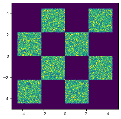
# Visualize the generated data distribution
samples = np.array(inf_train_gen(jax.random.PRNGKey(0), 500_000))

H=plt.hist2d(samples[:,0], samples[:,1], 300, range=((-5,5), (-5,5)))
cmin = 0.0
cmax = jnp.quantile(jnp.array(H[0]), 0.99).item()
norm = cm.colors.Normalize(vmax=cmax, vmin=cmin)

_ = plt.hist2d(samples[:,0], samples[:,1], 300, range=((-5,5), (-5,5)), norm=norm, cmap="viridis")

# set equal ratio of axes
plt.gca().set_aspect('equal', adjustable='box')
plt.show()

3. Model and Loss Definition

We define the score model (an MLP), the loss function, and the optimizer for training the diffusion model.

# Import diffusion model components and utilities
from gensbi.utils.model_wrapping import ModelWrapper
from gensbi.diffusion.path import EDMPath
from gensbi.diffusion.path.scheduler import EDMScheduler
from gensbi.diffusion.solver import SDESolver

# Define the MLP score model
class MLP(nnx.Module):
    def __init__(self, input_dim: int = 2, hidden_dim: int = 128, *, rngs: nnx.Rngs):
        self.input_dim = input_dim
        self.hidden_dim = hidden_dim

        din = input_dim + 1

        self.linear1 = nnx.Linear(din, self.hidden_dim, rngs=rngs)
        self.linear2 = nnx.Linear(self.hidden_dim, self.hidden_dim, rngs=rngs)
        self.linear3 = nnx.Linear(self.hidden_dim, self.hidden_dim, rngs=rngs)
        self.linear4 = nnx.Linear(self.hidden_dim, self.hidden_dim, rngs=rngs)
        self.linear5 = nnx.Linear(self.hidden_dim, self.input_dim, rngs=rngs)

    def __call__(self, x: jax.Array, t: jax.Array):
        x = jnp.atleast_2d(x)
        t = jnp.atleast_1d(t)
        if len(t.shape)<2:
            t = t[..., None]
            t = jnp.broadcast_to(t, (x.shape[0], t.shape[-1]))

        h = jnp.concatenate([x, t], axis=-1)

        x = self.linear1(h)
        x = jax.nn.gelu(x)

        x = self.linear2(x)
        x = jax.nn.gelu(x)

        x = self.linear3(x)
        x = jax.nn.gelu(x)

        x = self.linear4(x)
        x = jax.nn.gelu(x)

        x = self.linear5(x)

        return x

# Initialize the score model
hidden_dim = 512
F_model = MLP(input_dim=2, hidden_dim=hidden_dim, rngs=nnx.Rngs(0))

# Define optimizer and learning rate schedule parameters
PATIENCE = 10
COOLDOWN = 5
FACTOR = 0.5
RTOL = 1e-4
ACCUMULATION_SIZE = 100
MAX_LR = 0.5e-3
MIN_LR = 0
MIN_SCALE = MIN_LR / MAX_LR

# Set up optimizer with reduce-on-plateau schedule
nsteps = 10_000
nepochs = 5

multistep = 1

opt = optax.chain(
    optax.adaptive_grad_clip(10.0),
    optax.adamw(MAX_LR),
    reduce_on_plateau(
        patience=PATIENCE,
        cooldown=COOLDOWN,
        factor=FACTOR,
        rtol=RTOL,
        accumulation_size=ACCUMULATION_SIZE,
        min_scale=MIN_SCALE,
    ),
)
if multistep > 1:
    opt = optax.MultiSteps(opt, multistep)
optimizer = nnx.Optimizer(F_model, opt)

# Restore the model from checkpoint if requested
if restore_model:
    checkpointer = ocp.StandardCheckpointer()
    abs_model = nnx.eval_shape(lambda: MLP(input_dim=2, hidden_dim=hidden_dim, rngs=nnx.Rngs(0)))
    abs_state = nnx.state(abs_model)
    # Orbax API expects a tree of abstract `jax.ShapeDtypeStruct`
    # that contains both sharding and the shape/dtype of the arrays.
    abs_state = jax.tree.map(
        lambda a, s: jax.ShapeDtypeStruct(a.shape, a.dtype, sharding=s),
        abs_state, nnx.get_named_sharding(abs_state, mesh)
    )
    loaded_sharded = checkpointer.restore(checkpoint_dir + '/v1',
                                         target=abs_state)

    graphdef, abstract_state = nnx.split(abs_model)
    F_model = nnx.merge(graphdef, loaded_sharded)
    checkpointer.close()

4. Training Loop

This section defines the training and validation steps, and runs the training loop if enabled. Early stopping and learning rate scheduling are used for efficient training.

# Set batch size for training
batch_size = 1024

# Instantiate the diffusion path and loss function
path = EDMPath(scheduler=EDMScheduler())
loss_fn = path.get_loss_fn()

# Generate validation data
val_data = inf_train_gen(jax.random.PRNGKey(1), 512)

# Validation loss computation
@nnx.jit
def val_loss(model, key):
    x_1 = val_data
    sigma = path.sample_sigma(key, x_1.shape[0])
    path_sample = path.sample(key, x_1, sigma)
    batch = path_sample.get_batch()
    loss = loss_fn(model, batch)
    return loss

# Training step function
@nnx.jit
def train_step(F_model, optimizer, batch):
    grad_fn = nnx.value_and_grad(loss_fn)
    loss, grads = grad_fn(F_model, batch)
    optimizer.update(grads, value=loss)  # In-place updates.
    return loss

# Import tqdm for progress bars and set early stopping flag
from tqdm import tqdm
early_stopping = True

# Initialize training state and tracking variables
best_state = nnx.state(F_model)
best_val_loss_value = val_loss(F_model, jax.random.PRNGKey(0))
val_error_ratio = 1.1
counter = 0
cmax = 10
print_every = 100

loss_array = []
val_loss_array = []

rngs = nnx.Rngs(42)

# Main training loop (runs only if train_model=True)
if train_model:
    F_model.train()

    for ep in range(nepochs):
        pbar = tqdm(range(nsteps))
        l = 0
        v_l = 0
        for j in pbar:
            if counter > cmax and early_stopping:
                print("Early stopping")
                # restore the model state to the best found so far
                graphdef, abstract_state = nnx.split(F_model)
                F_model = nnx.merge(graphdef, best_state)
                break

            # Generate a batch of target data x_1 from the data generator
            x_1 = inf_train_gen(rngs.train_step(), batch_size)
            # Sample noise levels and create path sample
            sigma = path.sample_sigma(rngs.train_step(), x_1.shape[0])
            path_sample = path.sample(rngs.train_step(), x_1, sigma)
            batch = path_sample.get_batch()

            # Compute loss and update model parameters in-place
            loss = train_step(F_model, optimizer, batch)
            l += loss.item()

            # Compute validation loss for early stopping and LR scheduling
            v_loss = val_loss(F_model, rngs.val_step())
            v_l += v_loss.item()

            if j > 0 and j % 100 == 0:
                # Compute average training and validation loss over the last 100 steps
                loss_ = l / 100
                val_ = v_l / 100

                # Compute ratios for early stopping and best model tracking
                ratio1 = val_ / loss_
                ratio2 = val_ / best_val_loss_value

                # If validation loss is not diverging, update best state if needed
                if ratio1 < val_error_ratio:
                    if val_ < best_val_loss_value:
                        best_val_loss_value = val_
                        best_state = nnx.state(F_model)
                    elif ratio2 < 1.05:
                        best_state = nnx.state(F_model)

                    counter = 0
                else:
                    counter += 1

                # Update progress bar with current metrics
                pbar.set_postfix(
                    loss=f"{loss_:.4f}",
                    ratio=f"{ratio1:.4f}",
                    counter=counter,
                    val_loss=f"{val_:.4f}",
                )
                loss_array.append(loss_)
                val_loss_array.append(val_)
                l = 0
                v_l = 0

    F_model.eval()

# Save the trained model to checkpoint (if training was performed)
if train_model:
    checkpointer = ocp.StandardCheckpointer()
    model_state = nnx.state(F_model)
    checkpointer.save(checkpoint_dir + '/v1', model_state)
    checkpointer.close()

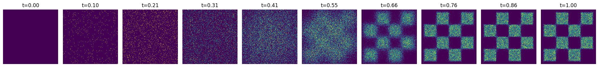
5. Sampling from the Model

In this section, we sample trajectories from the trained diffusion model and visualize the results at different time steps.

sample the model

# Set model to evaluation mode before sampling
F_model.eval()

# Sample trajectories from the model using SDE solver
nsteps = 30

norm = cm.colors.Normalize(vmax=50, vmin=0)

nsamples = 100_000  # batch size

key = jax.random.PRNGKey(0)

solver = SDESolver(score_model=F_model, path=path)  # create an SDESolver class
x_init = path.sample_prior(key, (nsamples,2) )  # sample initial points from the prior distribution
samples = solver.sample(key, x_init, nsteps=nsteps, return_intermediates=True)  # sample from the model

# Visualize the sampled trajectories at different time steps
T = np.linspace(0, 29, 10, endpoint=True, dtype=int)  # convert to numpy array

fig, axs = plt.subplots(1, len(T), figsize=(20,20))

for i,step in enumerate(T):
    H = axs[i].hist2d(samples[step,:,0], samples[step,:,1], 300, range=((-5,5), (-5,5)))

    cmin = 0.0
    cmax = jnp.quantile(jnp.array(H[0]), 0.99).item()

    norm = cm.colors.Normalize(vmax=cmax, vmin=cmin)

    _ = axs[i].hist2d(samples[step,:,0], samples[step,:,1], 300, range=((-5,5), (-5,5)), norm=norm, cmap="viridis")

    axs[i].set_aspect('equal')
    axs[i].axis('off')
    axs[i].set_title(f't={step/(nsteps-1):.2f}')

plt.tight_layout()
plt.show()

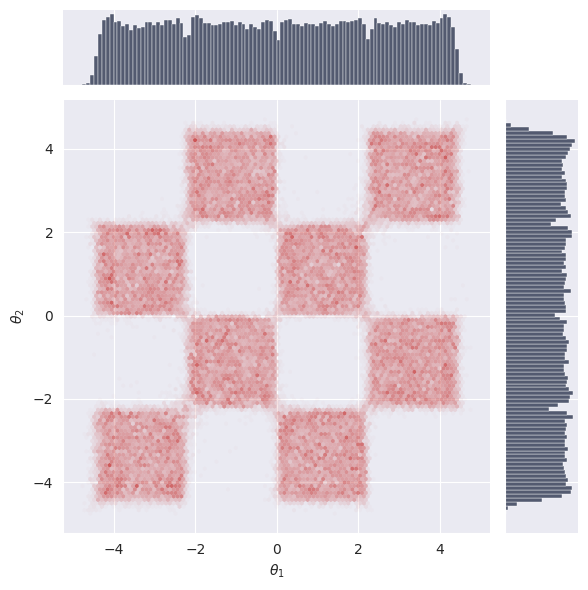
6. Marginal and Trajectory Visualization

We visualize the marginal distributions and sample trajectories from the diffusion model.

# Import plotting utilities for marginals and trajectories
from gensbi.utils.plotting import plot_trajectories, plot_marginals

# Plot the marginal distribution of the final samples
plot_marginals(samples[-1], plot_levels=False, gridsize=100)
plt.show()

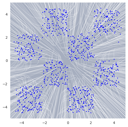
# Plot sampled trajectories
fig, ax = plot_trajectories(samples[:,:1000,:])
plt.xlim(-5, 5)
plt.ylim(-5, 5)
plt.grid(False)
plt.show()