Gaussian Linear Flux1Joint Flow Matching Example

---

This notebook demonstrates conditional flow-matching on the Gaussian Linear task using JAX and Flax.

# Check if running on Colab and install dependencies if needed
try:
    import google.colab
    colab = True
except ImportError:
    colab = False

if colab:
    # Install required packages and clone the repository
    %pip install "gensbi_examples[cuda12] @ git+https://github.com/aurelio-amerio/GenSBI-examples"
    !git clone https://github.com/aurelio-amerio/GenSBI-examples
    %cd GenSBI-examples/examples/sbi-benchmarks/two_moons

# load autoreload extension
%load_ext autoreload
%autoreload 2

import os
# select device

os.environ["JAX_PLATFORMS"] = "cuda"
# os.environ["JAX_PLATFORMS"] = "cpu"

## 1. Task & Data Preparation

In this section, we define the Gaussian Linear task, visualize reference samples, and create the training and validation datasets required for model learning. Batch size and sample count are set for reproducibility and performance.

restore_model=True
train_model=False

import orbax.checkpoint as ocp
# get the current notebook path
notebook_path = os.getcwd()
checkpoint_dir = os.path.join(notebook_path, "checkpoints")
os.makedirs(checkpoint_dir, exist_ok=True)

import matplotlib.pyplot as plt
import jax
import jax.numpy as jnp
from flax import nnx

from numpyro import distributions as dist
import numpy as np

from gensbi.utils.plotting import plot_marginals

from gensbi_examples.tasks import GaussianLinear
task = GaussianLinear()

/home/aure/miniforge3/envs/gensbi/lib/python3.12/site-packages/google/protobuf/runtime_version.py:98: UserWarning: Protobuf gencode version 5.28.3 is exactly one major version older than the runtime version 6.31.1 at grain/proto/execution_summary.proto. Please update the gencode to avoid compatibility violations in the next runtime release.
  warnings.warn(

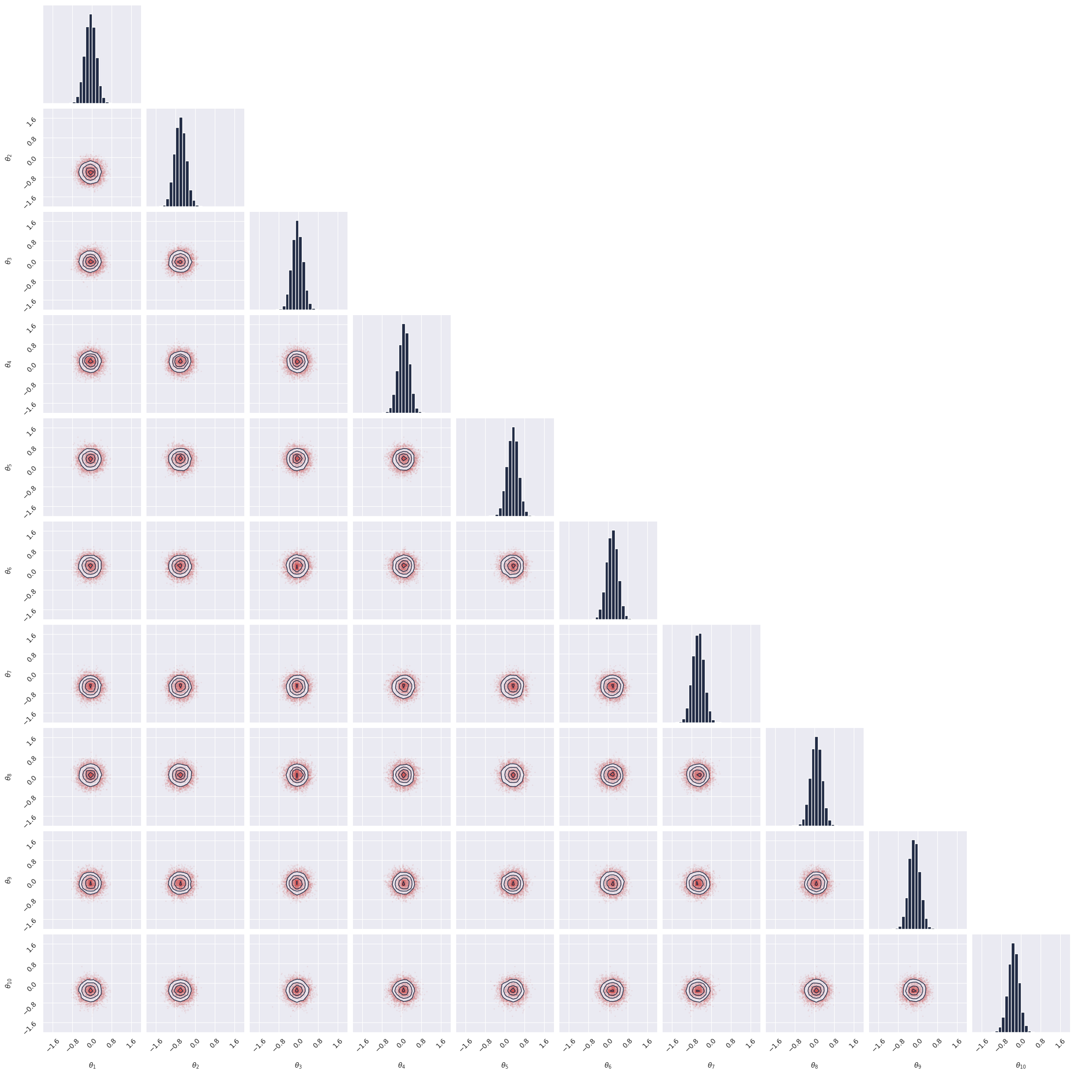
# reference posterior for an observation
obs, reference_samples = task.get_reference(num_observation=8)

# plot the triangle plot
plot_marginals(np.asarray(reference_samples, dtype=np.float32), gridsize=20, plot_levels=False, backend="seaborn")
plt.show()

# make a dataset
nsamples = int(1e5)

# Set batch size for training. Larger batch sizes help prevent overfitting, but are limited by available GPU memory.
batch_size = 4096
# Create training and validation datasets using the Gaussian Linear task object.
train_dataset = task.get_train_dataset(batch_size)
val_dataset = task.get_val_dataset()

# Create iterators for the training and validation datasets.
dataset_iter = iter(train_dataset)
val_dataset_iter = iter(val_dataset)

## 2. Model Configuration & Definition

In this section, we load the model and optimizer configuration, set all relevant parameters, and instantiate the Simformer model. Edge masks and marginalization functions are used for flexible inference and posterior estimation.

from gensbi.recipes import Flux1JointFlowPipeline

import yaml

# Path to the Simformer flow-matching configuration file.
config_path = f"{notebook_path}/config/config_flow_flux1joint.yaml"

# Load configuration parameters from YAML file.
with open(config_path, "r") as f:
    config = yaml.safe_load(f)

# Extract dimensionality information from the task object.
dim_theta = task.dim_theta  # Number of parameters to infer
dim_data = task.dim_data    # Number of observed data dimensions

dim_joint = task.dim_joint  # Joint dimension (for model input)

pipeline = Flux1JointFlowPipeline.init_pipeline_from_config(
        train_dataset,
        val_dataset,
        dim_theta,
        dim_data,
        config_path,
        checkpoint_dir,
    )

pipeline.restore_model()

WARNING:absl:CheckpointManagerOptions.read_only=True, setting save_interval_steps=0.
WARNING:absl:CheckpointManagerOptions.read_only=True, setting create=False.
WARNING:absl:Given directory is read only=/mnt/c/Users/Aure/Documents/GitHub/GenSBI-examples/examples/sbi-benchmarks/gaussian_linear/flow_flux1joint/checkpoints
WARNING:absl:CheckpointManagerOptions.read_only=True, setting save_interval_steps=0.
WARNING:absl:CheckpointManagerOptions.read_only=True, setting create=False.
WARNING:absl:Given directory is read only=/mnt/c/Users/Aure/Documents/GitHub/GenSBI-examples/examples/sbi-benchmarks/gaussian_linear/flow_flux1joint/checkpoints/ema

Restored model from checkpoint

## 3. Evaluation & Visualization

In this section, we evaluate the trained Simformer model by sampling from the posterior, and comparing results to reference data. We also compute and visualize the unnormalized log probability over a grid to assess model calibration and density estimation. These analyses provide insight into model performance and reliability.

### Section 3.1: Posterior Sampling

In this section, we sample from the posterior distribution using the trained model and visualize the results. Posterior samples are generated for a selected observation and compared to reference samples to assess model accuracy.

# we want to do conditional inference. We need an observation for which we want to ocmpute the posterior
def get_samples(idx, nsamples=10_000, use_ema=True, rng=None):
    observation, reference_samples = task.get_reference(idx)
    true_param = jnp.array(task.get_true_parameters(idx))

    if rng is None:
        rng = jax.random.PRNGKey(42)

    time_grid = jnp.linspace(0,1,100)

    samples = pipeline.sample(rng, observation, nsamples, use_ema=use_ema, time_grid=time_grid)
    return samples, true_param, reference_samples

samples, true_param, reference_samples =  get_samples(8)

samples.shape

(100, 10000, 10)

### Section 3.2: Visualize Posterior Samples

In this section, we plot the posterior samples as a 2D histogram to visualize the learned distribution and compare it to the ground truth.

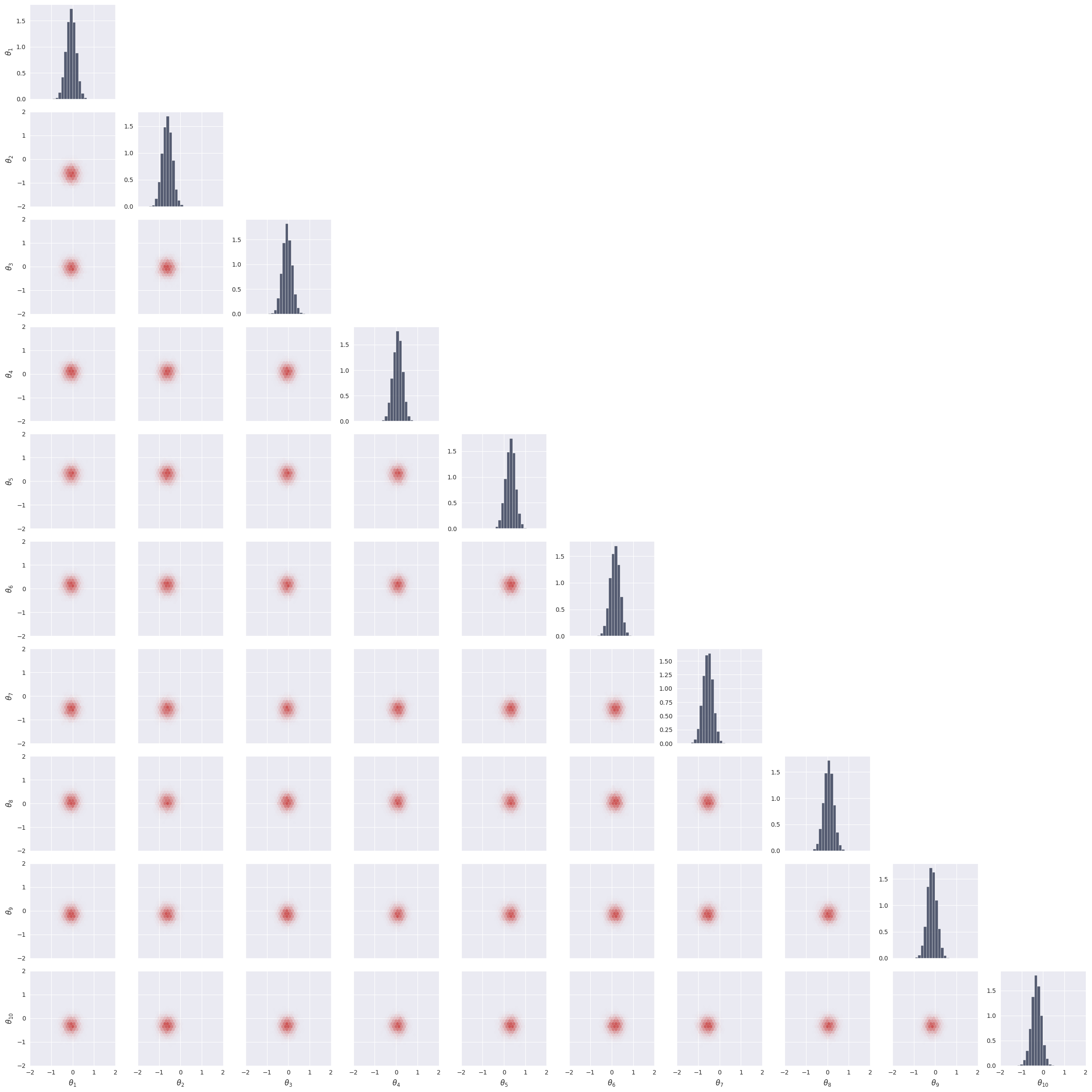
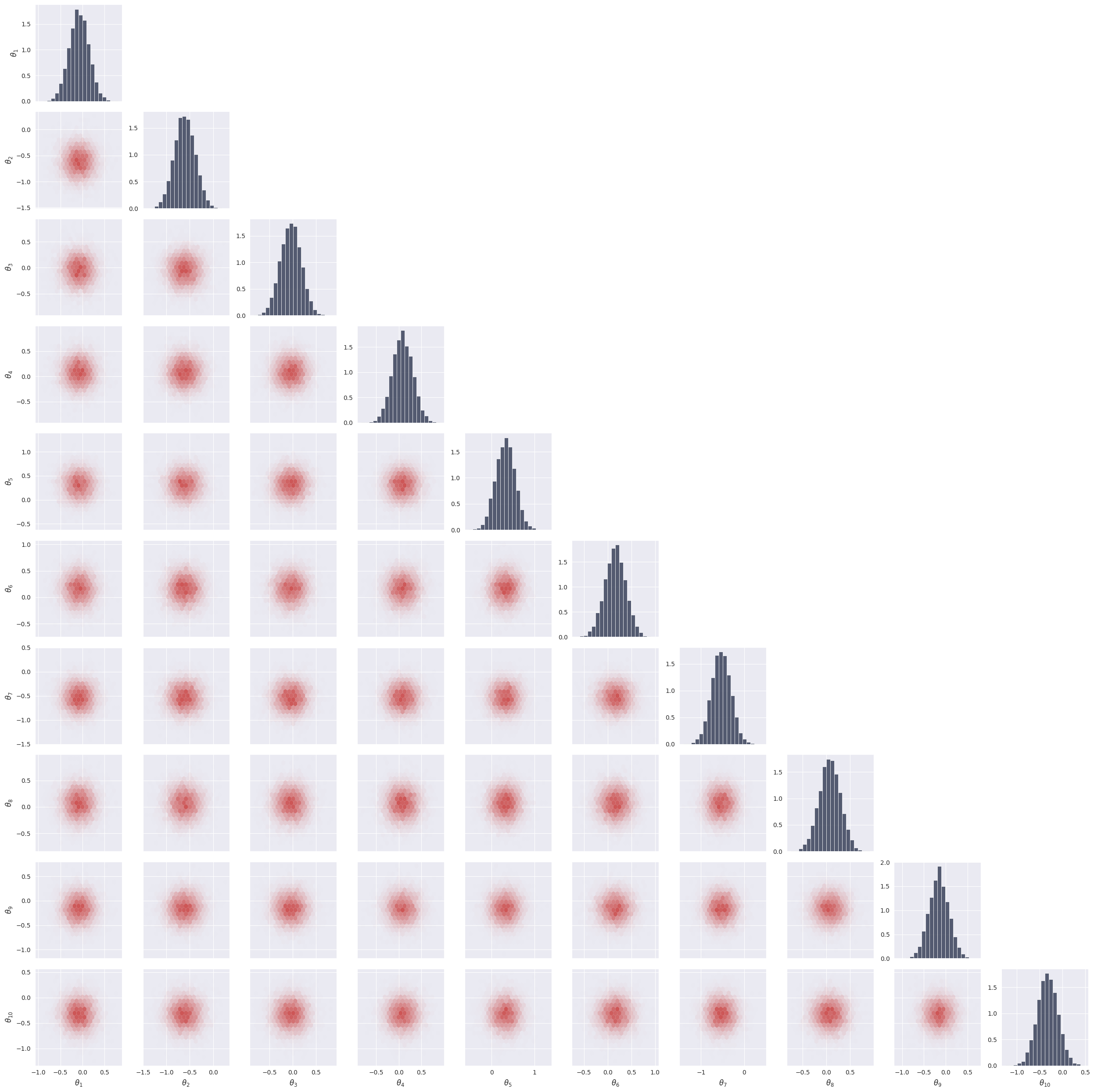
from gensbi.utils.plotting import plot_marginals

plot_marginals(samples[-1], plot_levels=False, gridsize=30, range=(-2,2))
plt.show()

# check how we set the ranges in the seaborn plot, it seems wrong
plot_marginals(samples[-1], plot_levels=False, backend="seaborn", gridsize=30, range=(-2,2))
# plt.text(1.05, 1.05, f"t = {1.0}", transform=plt.gca().transAxes)
plt.show()

<Figure size 640x480 with 0 Axes>