Flow Matching 2D Unconditional Example

This notebook demonstrates how to train and sample from a flow-matching model on a 2D toy dataset using JAX and Flax. We will cover data generation, model definition, training, sampling, and likelihood estimation.

1. Environment Setup

In this section, we set up the notebook environment, import required libraries, and configure JAX for CPU or GPU usage.

# Load autoreload extension for development convenience
%load_ext autoreload
%autoreload 2

The autoreload extension is already loaded. To reload it, use:
  %reload_ext autoreload

try: #check if we are using colab, if so install all the required software
    import google.colab
    colab=True
except:
    colab=False

if colab: # you may have to restart the runtime after installing the packages
    %pip install "gensbi_examples[cuda12] @ git+https://github.com/aurelio-amerio/GenSBI-examples"
    !git clone https://github.com/aurelio-amerio/GenSBI-examples
    %cd GenSBI-examples/examples

# Set training and model restoration flags
overwrite_model = False
restore_model = True  # Use pretrained model if available
train_model = False  # Set to True to train from scratch

Library Imports and JAX Backend Selection

# Import libraries and set JAX backend
import os
os.environ['JAX_PLATFORMS']="cuda" # select cpu instead if no gpu is available
# os.environ['JAX_PLATFORMS']="cpu"

from flax import nnx
import jax
import jax.numpy as jnp
import optax
from optax.contrib import reduce_on_plateau
import numpy as np

# Visualization libraries
import matplotlib.pyplot as plt
from matplotlib import cm

# Define the mesh for JAX sharding (for model restoration on CPU/GPU)
devices = jax.devices()
mesh = jax.sharding.Mesh(devices, axis_names=('data',)) # A simple 1D mesh

# Specify the checkpoint directory for saving/restoring models
import orbax.checkpoint as ocp
checkpoint_dir = f"{os.getcwd()}/checkpoints/flow_matching_2d_example"

import os
os.makedirs(checkpoint_dir, exist_ok=True)

if overwrite_model:
    checkpoint_dir = ocp.test_utils.erase_and_create_empty(checkpoint_dir)

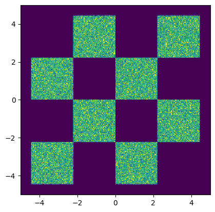
2. Data Generation

We generate a synthetic 2D dataset using JAX. This section defines the data generation functions and visualizes the data distribution.

# Define a function to generate 2D box data using JAX
import jax
import jax.numpy as jnp
from jax import random
from functools import partial

@partial(jax.jit, static_argnums=[1])  # type: ignore
def make_boxes_jax(key, batch_size: int = 200):
    """
    Generates a batch of 2D data points similar to the original PyTorch function
    using JAX.

    Args:
        key: A JAX PRNG key for random number generation.
        batch_size: The number of data points to generate.

    Returns:
        A JAX array of shape (batch_size, 2) with generated data,
        with dtype float32.
    """
    # Split the key for different random operations
    keys = jax.random.split(key, 3)
    x1 = jax.random.uniform(keys[0],batch_size) * 4 - 2
    x2_ = jax.random.uniform(keys[1],batch_size) - jax.random.randint(keys[2], batch_size, 0,2) * 2
    x2 = x2_ + (jnp.floor(x1) % 2)

    data = 1.0 * jnp.concatenate([x1[:, None], x2[:, None]], axis=1) / 0.45

    return data

# Infinite data generator for training batches
@partial(jax.jit, static_argnums=[1])  # type: ignore
def inf_train_gen(key, batch_size: int = 200):
    x = make_boxes_jax(key, batch_size)

    return x

# Visualize the generated data distribution
samples = inf_train_gen(jax.random.PRNGKey(0), 500_000)

H=plt.hist2d(samples[:,0], samples[:,1], 300, range=((-5,5), (-5,5)))
cmin = 0.0
cmax = jnp.quantile(jnp.array(H[0]), 0.99).item()
norm = cm.colors.Normalize(vmax=cmax, vmin=cmin)

_ = plt.hist2d(samples[:,0], samples[:,1], 300, range=((-5,5), (-5,5)), norm=norm, cmap="viridis")

# set equal ratio of axes
plt.gca().set_aspect('equal', adjustable='box')


plt.show()

3. Model and Loss Definition

We define the velocity field model (an MLP), the loss function, and the optimizer for training the flow-matching model.

# Import flow matching components and utilities
from gensbi.flow_matching.path.scheduler import CondOTScheduler
from gensbi.flow_matching.path import AffineProbPath
from gensbi.flow_matching.solver import ODESolver
from gensbi.utils.model_wrapping import ModelWrapper
from gensbi.flow_matching.loss import ContinuousFMLoss

# Define the MLP velocity field model
class MLP(nnx.Module):
    def __init__(self, input_dim: int = 2, hidden_dim: int = 128, *, rngs: nnx.Rngs):

        self.input_dim = input_dim
        self.hidden_dim = hidden_dim

        din = input_dim + 1

        self.linear1 = nnx.Linear(din, self.hidden_dim, rngs=rngs)
        self.linear2 = nnx.Linear(self.hidden_dim, self.hidden_dim, rngs=rngs)
        self.linear3 = nnx.Linear(self.hidden_dim, self.hidden_dim, rngs=rngs)
        self.linear4 = nnx.Linear(self.hidden_dim, self.hidden_dim, rngs=rngs)
        self.linear5 = nnx.Linear(self.hidden_dim, self.input_dim, rngs=rngs)

    def __call__(self, x: jax.Array, t: jax.Array, args=None):
        x = jnp.atleast_2d(x)
        t = jnp.atleast_1d(t)
        if len(t.shape)<2:
            t = t[..., None]
            t = jnp.broadcast_to(t, (x.shape[0], t.shape[-1]))

        h = jnp.concatenate([x, t], axis=-1)

        x = self.linear1(h)
        x = jax.nn.gelu(x)

        x = self.linear2(x)
        x = jax.nn.gelu(x)

        x = self.linear3(x)
        x = jax.nn.gelu(x)

        x = self.linear4(x)
        x = jax.nn.gelu(x)

        x = self.linear5(x)

        return x

# Initialize the velocity field model
hidden_dim = 512

# velocity field model init
vf_model = MLP(input_dim=2, hidden_dim=hidden_dim, rngs=nnx.Rngs(0))

# @markdown Define optimizer and learning rate schedule parameters
# @markdown Number of epochs to wait before resuming normal operation after the learning rate reduction:
PATIENCE = 10  # @param{type:"integer"}
# @markdown Factor by which to reduce the learning rate:
COOLDOWN = 5  # @param{type:"integer"}
# @markdown Relative tolerance for measuring the new optimum:
FACTOR = 0.5  # @param{type:"number"}
# @markdown Number of iterations to accumulate an average value:
ACCUMULATION_SIZE = 100
RTOL = 1e-4  # @param{type:"number"}
# @markdown learnign rate
MAX_LR = 1e-3  # @param{type:"number"}
MIN_LR = 0  # @param{type:"number"}
MIN_SCALE = MIN_LR / MAX_LR

# Set up optimizer with reduce-on-plateau schedule
nsteps = 10_000
nepochs = 10

multistep = 1 # if the GPU cannot support batch sizes of at least 4k, adjust this value accordingly to get the desired effective batch size

# warmup_schedule = optax.schedules.warmup_constant_schedule(1e-5, MAX_LR, warmup_steps=1000)

opt = optax.chain(
    optax.adaptive_grad_clip(10.0),
    # optax.adamw(warmup_schedule),
    optax.adamw(MAX_LR),
    reduce_on_plateau(
        patience=PATIENCE,
        cooldown=COOLDOWN,
        factor=FACTOR,
        rtol=RTOL,
        accumulation_size=ACCUMULATION_SIZE,
        min_scale=MIN_SCALE,
    ),
)
if multistep > 1:
    opt = optax.MultiSteps(opt, multistep)
optimizer = nnx.Optimizer(vf_model, opt)

# Restore the model from checkpoint if requested
if restore_model:
    checkpointer = ocp.StandardCheckpointer()
    abs_model = nnx.eval_shape(lambda: MLP(input_dim=2, hidden_dim=hidden_dim, rngs=nnx.Rngs(0)))
    abs_state = nnx.state(abs_model)
    # Orbax API expects a tree of abstract `jax.ShapeDtypeStruct`
    # that contains both sharding and the shape/dtype of the arrays.
    abs_state = jax.tree.map(
    lambda a, s: jax.ShapeDtypeStruct(a.shape, a.dtype, sharding=s),
    abs_state, nnx.get_named_sharding(abs_state, mesh)
    )
    loaded_sharded = checkpointer.restore(checkpoint_dir + '/v1',
                                        target=abs_state)

    graphdef, abstract_state = nnx.split(abs_model)
    vf_model= nnx.merge(graphdef, loaded_sharded )
    checkpointer.close()

4. Training Loop

This section defines the training and validation steps, and runs the training loop if enabled. Early stopping and learning rate scheduling are used for efficient training.

# Set batch size for training
batch_size = 1024

from numpyro import distributions as dist

# define the prior distribution, in this case a 2D gaussian with zero mean and unit variance
p0 = dist.Independent(dist.Normal(jnp.zeros(2), jnp.ones(2)), 1)

# Instantiate the affine path and loss function
path = AffineProbPath(scheduler=CondOTScheduler())

loss_fn = ContinuousFMLoss(path)

@nnx.jit
def train_step(vf_model, optimizer, batch):
    grad_fn = nnx.value_and_grad(loss_fn)
    loss, grads = grad_fn(vf_model, batch)
    optimizer.update(grads, value=loss)  # In-place updates.

    return loss

# Generate validation data
val_data = inf_train_gen(jax.random.PRNGKey(1), 512)

# Validation loss computation
@nnx.jit
def val_loss(model, key):
    subkey2, subkey3 = jax.random.split(key, 2)
    x_1 = val_data
    x_0 = p0.sample(subkey2, (x_1.shape[0],))
    t = jax.random.uniform(subkey3, x_1.shape[0])

    batch = (x_0, x_1, t)
    return loss_fn(model, batch)

# Import tqdm for progress bars and set early stopping flag
from tqdm import tqdm
early_stopping = True

# Initialize training state and tracking variables
best_state = nnx.state(vf_model)
best_val_loss_value = val_loss(vf_model, jax.random.PRNGKey(0))
val_error_ratio = 1.1
counter = 0
cmax = 10
print_every = 100

loss_array = []
val_loss_array = []

rngs = nnx.Rngs(42)

# Main training loop (runs only if train_model=True)
if train_model:
    vf_model.train()

    for ep in range(nepochs):
        pbar = tqdm(range(nsteps))
        l = 0
        v_l = 0
        for j in pbar:
            if counter > cmax and early_stopping:
                print("Early stopping")
                # restore the model state to the best found so far
                graphdef, abstract_state = nnx.split(vf_model)

                vf_model = nnx.merge(graphdef, best_state)
                break

            # Generate a batch of target data x_1 from the data generator
            x_1 = inf_train_gen(rngs.train_step(), batch_size=batch_size) # sample data
            # Sample x_0 from the standard normal prior, matching the shape of x_1
            x_0 = p0.sample(rngs.train_step(), (x_1.shape[0],))
            # Sample t uniformly in [0, 1] for each data point in the batch
            t = jax.random.uniform(rngs.train_step(), x_1.shape[0])

            # Prepare the batch tuple for the loss function
            batch = (x_0, x_1, t)
            # Compute loss and update model parameters in-place
            loss = train_step(vf_model, optimizer, batch)  # update model parameters
            l += loss.item()

            # Compute validation loss for early stopping and LR scheduling
            v_loss = val_loss(vf_model, rngs.val_step())
            v_l += v_loss.item()

            if j > 0 and j % 100 == 0:
                # Compute average training and validation loss over the last 100 steps
                loss_ = l / 100
                val_ = v_l / 100

                # Compute ratios for early stopping and best model tracking
                ratio1 = val_ / loss_
                ratio2 = val_ / best_val_loss_value

                # If validation loss is not diverging, update best state if needed
                if ratio1 < val_error_ratio:
                    if val_ < best_val_loss_value:
                        best_val_loss_value = val_
                        best_state = nnx.state(vf_model)
                    elif ratio2 < 1.05:
                        best_state = nnx.state(vf_model) # still update the best state if the ratio is below 1.05

                    counter = 0
                else:
                    # If validation loss is diverging, increment early stopping counter
                    counter += 1

                # Update progress bar with current metrics
                pbar.set_postfix(
                    loss=f"{loss_:.4f}",
                    ratio=f"{ratio1:.4f}",
                    counter=counter,
                    val_loss=f"{val_:.4f}",
                )
                loss_array.append(loss_)
                val_loss_array.append(val_)
                l = 0
                v_l = 0

    vf_model.eval()

# Save the trained model to checkpoint (if training was performed)
if train_model:
    checkpointer = ocp.StandardCheckpointer()
    model_state = nnx.state(vf_model)
    checkpointer.save(checkpoint_dir + '/v1.1', model_state)
    checkpointer.close()

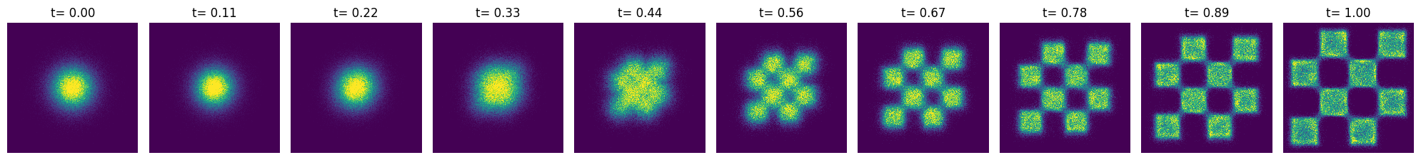
5. Sampling from the Model

In this section, we sample trajectories from the trained flow-matching model and visualize the results at different time steps.

sample the model

# Set model to evaluation mode before sampling
vf_model.eval()

# Wrap the model for ODE solver compatibility
vf_wrapped = ModelWrapper(vf_model)

# Sample trajectories from the model using ODE solver
step_size = 0.05

norm = cm.colors.Normalize(vmax=50, vmin=0)

batch_size = 500_000  # batch size
T = jnp.linspace(0,1,10)  # sample times

x_init = p0.sample(jax.random.PRNGKey(0), (batch_size, ))  # initial conditions
solver = ODESolver(velocity_model=vf_wrapped)  # create an ODESolver class
sol = solver.sample(time_grid=T, x_init=x_init, method='Dopri5', step_size=step_size, return_intermediates=True)

# Visualize the sampled trajectories at different time steps
sol = np.array(sol)  # convert to numpy array
T = np.array(T)  # convert to numpy array

fig, axs = plt.subplots(1, 10, figsize=(20,20))

for i in range(10):
    H = axs[i].hist2d(sol[i,:,0], sol[i,:,1], 300, range=((-5,5), (-5,5)))

    cmin = 0.0
    cmax = jnp.quantile(jnp.array(H[0]), 0.99).item()

    norm = cm.colors.Normalize(vmax=cmax, vmin=cmin)

    _ = axs[i].hist2d(sol[i,:,0], sol[i,:,1], 300, range=((-5,5), (-5,5)), norm=norm, cmap="viridis")

    axs[i].set_aspect('equal')
    axs[i].axis('off')
    axs[i].set_title('t= %.2f' % (T[i]))

plt.tight_layout()
plt.show()

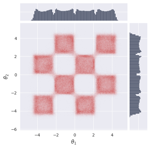
6. Marginal and Trajectory Visualization

We visualize the marginal distributions and sample trajectories from the model.

# Import plotting utility for marginals
from gensbi.utils.plotting import plot_marginals

# Plot the marginal distribution of the final samples
plot_marginals(sol[-1], plot_levels=False, gridsize=100)
plt.show()

# Sample and visualize trajectories with finer time resolution
batch_size = 1000
T = jnp.linspace(0,1,50)  # sample times

x_init = p0.sample(jax.random.PRNGKey(0), (batch_size, ))  # initial conditions
solver = ODESolver(velocity_model=vf_wrapped)  # create an ODESolver class
sol = solver.sample(time_grid=T, x_init=x_init, method='Dopri5', step_size=step_size, return_intermediates=True)

# Import plotting utility for trajectories
from gensbi.utils.plotting import plot_trajectories

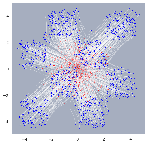
# Plot sampled trajectories
fig, ax = plot_trajectories(sol)
plt.grid(False)
plt.show()

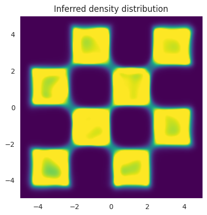
7. Likelihood Estimation

This section demonstrates how to estimate and visualize the likelihood of the model on a grid of points in 2D space.

sample the likelihood

# Import numpyro distributions for likelihood computation
import numpyro.distributions as dist

# Prepare grid for likelihood evaluation
T = jnp.array([1., 0.])  # sample times
grid_size = 200
x_1 = jnp.meshgrid(jnp.linspace(-5, 5, grid_size), jnp.linspace(-5, 5, grid_size))
x_1 = jnp.stack([x_1[0].flatten(), x_1[1].flatten()], axis=1)

# log_prob of the prior distribution
# Note: p0 is defined as an isotropic Gaussian with zero mean and unit variance
gaussian_log_density = p0.log_prob

# Compute unnormalized log-likelihood using the ODE solver
sampler = solver.get_unnormalized_logprob(time_grid=[1.0,0.0], method='Dopri5', step_size=step_size, log_p0=gaussian_log_density)

exact_log_p = sampler(x_1)

# Visualize the model likelihood on the 2D grid
likelihood = np.array(jnp.exp(exact_log_p[-1,:]).reshape(grid_size, grid_size))

cmin = 0
cmax = 1/40.5 # the domain goes from -4.5 to 4.5. The total area is (4.5*2)**2. Since only half of the area is covered by the data likelihood, we divide by 2 -> (4.5*2)**2 / 2 = 40.5. As Such 1/40.5 is the max theoretical likelihood value
norm = cm.colors.Normalize(vmax=cmax, vmin=cmin)

# Create the figure and axis objects explicitly
fig, ax = plt.subplots()

likelihood = np.array(jnp.exp(exact_log_p[-1,:]).reshape(grid_size, grid_size))

norm = cm.colors.Normalize(vmax=cmax, vmin=cmin)

im = ax.imshow(likelihood, extent=(-5, 5, -5, 5), origin='lower', cmap='viridis', norm=norm)
ax.set_title('Model Likelihood')

plt.grid(False)
plt.show()